|
Recursion in Nature, Mathematics and Art
Anne M. Burns Department of Mathematics Long Island University C.W. Post Campus Brookville, NY 11548
Abstract
This paper illustrates a number of ways that recursion and replacement rules can be used to create aesthetically pleasing computer generated pictures. Starting with imitation of forms found in nature, we move to more abstract designs, first designs derived from the nature imitations, and finally a purely abstract example.
1. Introduction
"In order to understand recursion, one must first understand recursion", from Wikipedia, the free encyclopedia
Many of the forms and shapes found in nature exhibit some form of self-similarity; the larger form appears to contain smaller copies of itself at different scales. Examples abound in the plant world; we see it also in mountains, clouds, the branching structure of rivers and blood vessels, patterns on animal skins, etc. Nature imposes restrictions on growth rules, but that doesn’t mean that the artist needs to. First imitating the forms and shapes in nature, the artist finds herself changing a shape, a scale or a color to produce a more abstract but visually appealing picture. We will start with algorithms that produce imitations of forms found in nature; next we combine them into what a colleague of mine termed "Mathscapes", and finally we will abstract the forms into visually appealing designs.
In mathematics and computer science a recursive function is a function that calls itself; by calling itself more than once a function can produce multiple copies of itself. This makes it an excellent technique for creating figures which are defined by "replacement" rules. Consider the following examples of replacement rules: In each of Figures 1 and 2, start with the leftmost figure. Then replace it by the second figure. This gives you the replacement rule. For example, in Figure 1 start with a line segment. At step 2 replace the line segment with 5 line segments as pictured, each 1/3 the length of the original. At step n replace each segment in step n-1 with a reduced copy of the step n-1 figure.
|
|
Figure 1: Example of a replacement rule
|
|
|
|
|
Figure 2: A geometric replacement rule
In Figure 3 the replacement rule is a little different; it is an example of a random displacement rule. At each step a random number is multiplied by a scale factor and then added to or subtracted from the average of the height at the left endpoint and the height at the right endpoint; the result is assigned to the height of the midpoint. Figure 4 shows the result of carrying out the rule until the left and right endpoints of each interval are the same. To produce more realistic looking natural forms we make much use of random numbers; in the example in Figure 1, instead of each line segment being 1/3 the length the length of the segments in the previous step we could make the line length a function of a Gaussian random variable with mean 1/3.
|
|
|
|
Figure 3: A random replacement rule

|
Figure 4: Result of replacement rule in Figure 3
2. Imitating forms found in nature
2.1. Plant forms.
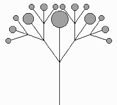
We start with plant forms; the technique of replacement rules could almost have been invented by observing an abstract tree structure. There are many excellent publications describing various models of plant growth. All involve some sort of recursion. Teaching computer graphics, I was on the lookout for examples of recursion and examples that illustrate the uses of simple trigonometry. In [8] I found simple stick diagrams of the common inflorescences; a few of them are shown in Figure 5.
 |
 |
|
 |
 |
 |
|
|
|
|
|
|
|
Figure 5: Some common inflorescences
Figure 6 shows the compounding of some of the inflorescences. These pictures were all done with simple recursion.
|
|
|
|
|
|
|
|
|
Figure 6: Compound inflorescences
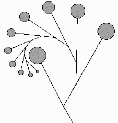
Figure 7 shows some imaginary inflorescences obtained by using random numbers to vary segment lengths and angles and taking artistic liberties with the above.
 |
 |
 |
 |
Figure 7: Imaginary inflorescences
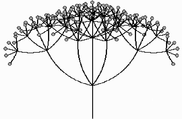
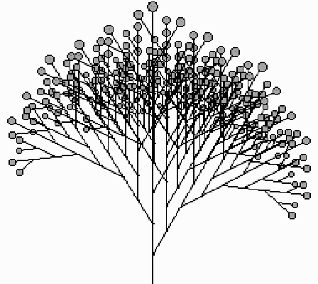
Another model for plants can be found in the article by deReffye et al [6]. In this model at each stage of growth a "bud" can do one of three things: (1) branch, (2) flower and ultimately die or (3) sleep (do nothing until the next stage). A probability is assigned to each of the three outcomes, such that the probabilities add up to 1. We start with a single bud; at each stage, for each bud that is still alive, we generate a random number between 0 and 1; the number determines the next state of that bud. For added realism we can make the probabilities functions of time, so that at later stages the probability of a bud dying is higher. Figure 8 shows three imaginary "trees" using a branching number of 2, that is, when a node branches it produces two new branches. The exact same program drew the three trees; using probabilities and random numbers we can make it look as if the three trees come from the same family, but are not identical.
|
Figure 8: Trees modeled using deReffye’s method
Another of my favorite ways to model botanical growth is a method called L-systems, or string rewriting. It was discovered by Aristid Lindenmayer, a Dutch biologist who had the remarkable idea of using concepts from formal language theory to describe plant growth, and developed by Premislaw Prusinciewicz [9]. In this model each geometric part of the plant is assigned a character. Here is a simple example: let I represent an internode, L a leaf and F a flower. We use brackets and parentheses to indicate branches. Square brackets enclose a branch to the left, parentheses enclose a branch to the right. For example, the string of characters I[I[L](L)IF]I(II(L)IF)IF might represent the imaginary plant in Figure 9a. At each stage we use a set of rewriting rules (productions) to successively replace each character by a string of characters. Figure 9 illustrates several stages in the development of an imaginary plant using this method.
|
|
|
|
|
|
|
|
|
Figure 9: Stages in an imaginary plant resulting from string rewriting
Another method of modeling plant growth and other branching phenomena uses a stochastic matrix of probabilities; this method is reminiscent of a Markov chain. Space considerations preclude a description here, but the interested reader can find more in [5].
2.2. Mountains and clouds.
The midpoint displacement rule illustrated in Figures 3 and 4 can be extended to a two dimensional model in which we obtain a height field over a two-dimensional grid. We can use this to model both mountains and clouds. To model clouds, we assign a ramp of colors to the heights, while to model mountains we use some trigonometry and calculus to project the three dimensional height field onto a two dimensional surface.
First we outline the recursive midpoint algorithm for generating the height field. We start with a 2n+1 by 2n+1 grid of points in the plane, where n could be 9, for example, for a 513 by 513 grid. We assign a number to each of the 4 corner points. At step 1 we assign a value to the point labeled 1 in Figure 10a; the value is the average of the numbers at the 4 corner points plus a random number. At step 2 we assign values to the points labeled 2 in Figure10b, by taking the average of the three closest previously assigned points plus a random amount. Figures 10c and 10d show the order in which the next several points are assigned. At each stage the random amount is scaled down.
Once the height field is generated we can render it as three dimensional mountains using some calculus and trigonometry, illustrated in Figure 11a, or we can assign a continuous ramp of colors to the heights and render it as clouds, illustrated in Figure 11b. By changing the scale factor that we use in scaling down the random amount that we add at each stage, we can produce sharp fractal-like mountains and clouds or soft rounded mountains and cumulus clouds.
 |
 |
 |
 |
|
|
|
|
|
Figure 10: Can you guess which pixels will be assigned at Stage 5?
|
|
|
|
|
Figure 11
3. Mathscapes
|
|
Figure 12: "Mathscape" |
Soft, rounded mountains, like those found in Vermont, can also be produced by using sums of trigonometric functions with randomly assigned coefficients, which can then be projected onto a two-dimensional picture using the same rendering technique that we used for the fractal mountains generated by the midpoint algorithm.
In Figure 12, "Mathscape", I have combined the recursive algorithms for clouds, mountains and various imaginary plant forms into one picture.
4. "Persian" Rugs
The midpoint algorithm that produced the clouds and mountains can also be used to generate abstract designs that resemble Persian rugs. Instead of adding a random amount at each stage, we add an integer amount based on some function of the previously assigned values. Then to each integer we assign a color. For example, in the first stage of the recursion we assigned a value to the middle point based on the values assigned to the corner points. To design a "Persian" rug, since we want symmetry, we would initially assign the same integer value to the four corner points. To get the value for the center point we let x1 be the value assigned to the upper left corner, x2 the value assigned to the upper right corner, x3 the value assigned to the lower left corner and x4 the value assigned to the lower right corner. An example of a function that assigned the value to the midpoint might be f(x1, x2, x3, x4) = (x1 + x2 + x3 + x4)/ 3 mod 17. Actually I discovered a simpler algorithm [4] which goes something like this: assign integers to a set of k+1 colors. Color all points on the borders of the grid color j, j € {0,..,k}. As in the first method, make up a function f of 4 integers that returns an integer. Apply f to the 4 corner points resulting in an integer m between 0 and k. Color all points on the two lines connecting the midpoints of the opposite borders the new color m, then recursively repeat the process for the four new squares until all pixels have been colored in. Some examples can be seen in Figure 13.
|
|
|
Figure 13: "Persian" recursion
5. Using recursion to produce abstract designs
Looking at the replacement rule illustrated in Figure 2 we see that it seems to say: start with a circle, replace the circle with four smaller circles tangent to each other and tangent to the original circle. Then at the next stage repeat the operation with each of the new circles. We can generalize this procedure using what mathematicians call an Iterated Function System (IFS). This is a collection of n ≥ 2 contraction mappings of a set into itself. For example, suppose we have a collection of transformations {Tj}, each one mapping a circle to a smaller circle contained in the original circle. A recursive algorithm for drawing a design such as the one in Figure 2 might look like this:
    Function Recurse(step, center, radius )
    {
        If (step == 0)
        {
            Draw the circle with center center and radius radius;
        }
        else
        {
            for (j = 1; j <= number of transformations; j++)
            {
                find newcenter, newradius, the center and radius of Tj(C);
                Recurse(step-1, newcenter, newradius);
            }
        }
    }
The limit set of an IFS is the set of points that is invariant under all compositions of the contraction mappings. In general it is a fractal. For a complete theory see [1]. To produce interesting designs, we can just carry out the recursion for a few steps. For iterated function systems involving circles it is convenient to use Möbius transformations which map circles to circles.
|
|
|
Figure 14: Iterated Möbius transformations
|
|
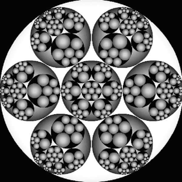
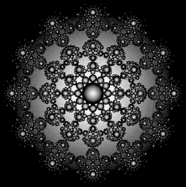
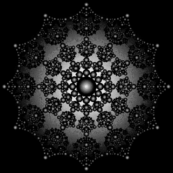
Figure 15: Showing only selected stages of the recursion and using color in imaginative ways
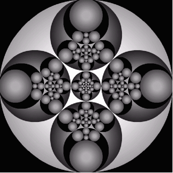
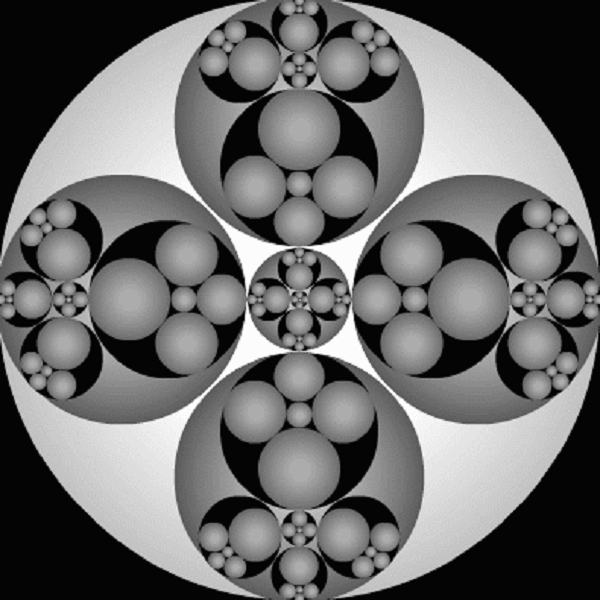
If we carry out the recursion suggested by Figure 2, we find that the design is not particularly interesting. The transformations that take the original circle into the four smaller circles are affine transformations; they shrink and then translate the original circle, but do not distort it. We can generate more varied pictures if we alter the original transformations by composing them with Möbius transformations from the unit circle group. Transformations from the unit circle group map the unit circle to itself, expanding it or contracting distances along the circle depending on two complex parameters. As we iterate the distortions propagate, producing more varied and interesting designs. In Figure 14 we see the effect of changing the parameters. We have also added to the replacement rules a central circle that is tangent to the other four and in the rightmost picture we have increased the number of circles tangent to the original circle to six. Figure 15 shows two renderings where we increase the number of circles to thirteen, show only selected stages of the recursion and use color in imaginative ways.
6. Conclusion
Recursion is a great way to get students interested in mathematics and computer graphics. Students are always amazed at how what looks like a really complicated figure can be produced in a few lines of code. All the figures in this paper except string-rewriting were produced using simple recursion, that is, a single recursive function that calls itself two or more times. Nearly all programming languages support recursive functions. For future investigations we might explore using a recursive chain. A recursive chain is a set of two or more functions that call each other.
|
Figure 16: Overlapping circles
References
Fractals Everywhere, Academic Press, Inc., San Diego, 1988
[2] A. Burns, "Evolution of Math into Art via Möbius transformations", Math+Art = X Proceedings. Boulder, CO, June 2005 (forthcoming)
[3] A. Burns, "Recursion: Real and Imaginary Inflorescences", The UMAP Journal, Vol. 21, No. 4, Winter 2000
[4] A. Burns, " ‘Persian’ Recursion", Mathematics Magazine, Vol. 70, No. 3, June 1997
[5] A. Burns, "Modeling Trees with Stochastic Matrices", The College Mathematics Journal, Vol. 29, No. 3, May 1998
[6] P. deReffye, C. Edelin, J. Francon, M. Jaeger, C. Puech, "Plant Models Faithful to Botanical Structure and Development", Computer Graphics, Vol. 22, No. 4, August 1988
[7] D. Mumford, C. Series and D. Wright, Indra’s Pearls: the Vision of Felix Klein, Cambridge University Press, 2002
[8] C.L. Porter, Taxonomy of Flowering Plants, W.H. Freeman, San Fransisco, 1967
[9] P. Prusinkiewicz and A. Lindenmayer, The Algorithmic Beauty of Plants, Springer-Verlag, New York, 1990